

Simulated linguistic data for teaching and learning statistics in R.
simling has 56 data sets. 54 come from 20 branches of linguistics, from acoustic phonetics to language evolution; the other two are a meta-analysis and a messy export for data cleaning. Responses include reaction times, acoustic measurements, ratings, counts, binary and multi-category outcomes, time series and EEG.
Use them in class or to learn on your own. If you are planning a study, you can see what its data will look like and try out the analysis first.
Every data set is simulated, so the true effects are known and you can check whether your model recovers them. Each help page (?vowel_duration) gives the variables, the true model and example analyses. The simulation code is in data-raw/.
Installation
Install simling from R-universe:
install.packages("simling", repos = c("https://mcanzi.r-universe.dev", "https://cloud.r-project.org"))Usage
Loading and plotting a data set
Each data set loads with the package. Here is the pupil data, with single trials and the mean in each condition:
library(simling)
library(ggplot2)

pupil_noise
?pupil_noise

ggplot(pupil_noise, aes(time, pupil, colour = condition)) +
  geom_line(aes(group = trial_id), alpha = 0.08) +
  stat_summary(fun = mean, geom = "line", linewidth = 1.2) +
  scale_colour_manual(values = c(quiet = "#4f86b5", noise = "#e0735a")) +
  labs(x = "Time from stimulus onset (ms)",
       y = "Pupil size (baseline-corrected)") +
  theme_minimal()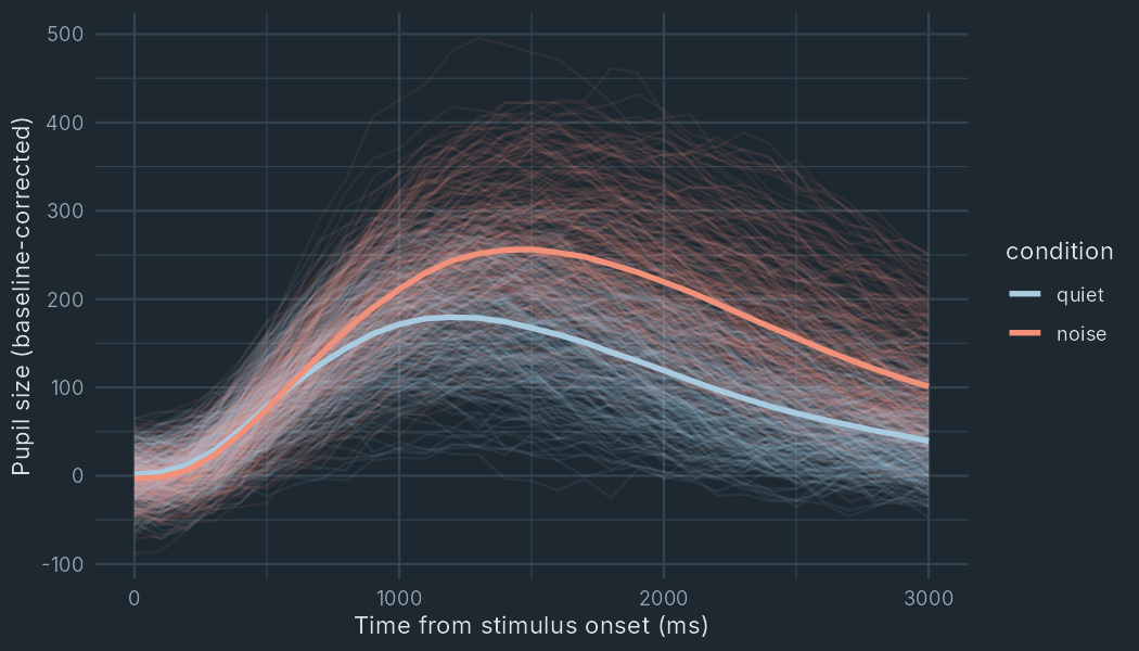
In the true model on the help page, the pupil peaks 90 units higher and 250 ms later in noise than in quiet. In the plotted means the difference is about 77 units and 300 ms. The help page suggests a GAMM with autocorrelated residuals for estimating these differences.
Checking an analysis against the true model
The help page of vowel_duration gives the model the data come from: vowels are 150 ms long before voiceless consonants and 20 ms longer before voiced ones, with by-speaker and by-word variation. A mixed model fitted to the data recovers these values:
library(lme4)
m <- lmer(duration ~ voicing + (1 + voicing | speaker) + (1 | word),
          data = vowel_duration)
summary(m)| True value | Estimate | |
|---|---|---|
| Intercept (voiceless) | 150 ms | 155.5 ms |
| Effect of voicing | 20 ms | 20.5 ms |
| By-speaker SD of the intercept | 25 ms | 24.5 ms |
| By-speaker SD of the voicing effect | 12 ms | 7.6 ms |
| By-word SD of the intercept | 15 ms | 12.6 ms |
| Residual SD | 20 ms | 20.0 ms |
The estimates differ from the true values because each data set is one random sample from its model; with only 16 speakers, the SD of the voicing effect is the hardest to estimate. Students can also fit a wrong model, for example one without by-speaker slopes, and see what changes.
Finding a data set
To find a data set for a lesson, simling_datasets() lists all of them with their branch, language, size, response and topic:
library(dplyr)
simling_datasets() |> filter(branch == "Psycholinguistics")
simling_datasets() |> filter(grepl("counts", response))
Factors and reference levels
Every categorical column is a factor. Its first level is the reference level: the baseline condition, such as "voiceless" in vowel_duration or "grammatical" in agreement_attraction. IDs such as participants, speakers and words are factors too. Binary outcomes coded 0/1 and rating scales are numeric. The one exception is messy_export, which keeps the text columns of a raw export so that students can clean it.
Data sets
| Branch | Data set | Language | Rows | Response | Topic |
|---|---|---|---|---|---|
| Phonetics | formants |
– | 120 | continuous | Normalisation, z-scores |
vowel_voicing |
English | 120 | continuous | Two groups, t-tests | |
speech_styles |
– | 150 | continuous | Categorical predictors with three levels | |
style_voicing |
– | 160 | continuous | Categorical × categorical interaction | |
vowel_duration |
– | 384 | continuous | Mixed models, random slopes | |
korean_stops |
Korean | 1,440 | continuous | Cluster analysis, sound change | |
price_f2 |
English (L1 and L2) | 2,200 | trajectories | GAMs and GAMMs | |
mandarin_tones |
Mandarin | 4,224 | trajectories | Contour shape, speaker normalisation | |
vot_identification |
English, Spanish | 1,224 | binomial counts | Psychometric curves, category boundaries | |
| Phonology | hungarian_harmony |
Hungarian | 4,200 | binary | Mixed logistic regression, wug tests |
| Prosody | tobi_agreement |
German | 456 | labels from two coders | Inter-rater agreement, kappa |
rhythm_metrics |
6 languages | 1,200 | continuous | Variance partitioning, speech rate | |
speech_to_song |
English | 516 | binary, ordinal | Mixed logistic and ordinal models | |
| Psycholinguistics | rt_frequency |
– | 200 | RT, binary | Data wrangling |
freq_length |
– | 400 | RT | Continuous × continuous interaction | |
l2_frequency |
– | 400 | RT | Continuous × categorical interaction | |
lexical_decision |
– | 800 | RT | Mixed models, crossed random effects | |
lexical_decision_l2 |
German (L1 and L2) | 1,200 | RT | Mixed models with interactions, figures | |
naming_pilot |
German | 1,200 | naming latency | Power analysis by simulation | |
lexical_accuracy |
Italian | 1,800 | binary | Mixed logistic regression | |
zipf_rt |
– | 2,000 | RT | Skewed predictors, log transformations | |
disfluencies |
Italian | 2,400 | counts, many zeros | Zero-inflated count models | |
megastudy |
– | 6,000 | RT, proportion | Large item-level data, non-linear effects | |
pupil_noise |
– | 17,856 | trajectories | GAMMs, autocorrelation | |
n400 |
German | 21,600 | ERP amplitude | EEG, topography, continuous predictors | |
visual_world |
English | 23,040 | samples per object | Eye tracking, time-course analysis | |
reading_skipping |
English | 1,512 | binary, durations | Skipping and fixation times, missing by design | |
| Syntax | agreement_attraction |
English | 1,280 | eye-tracking measures, binary | Reading measures, missing data |
acceptability |
English | 1,536 | 7-point ratings | Ordinal regression | |
german_relatives |
German | 13,824 | reading times | Self-paced reading, region-by-region analysis | |
| Morphology | german_plurals |
German | 2,880 | five categories | Multinomial regression, wug tests |
| Semantics and pragmatics | scalar_implicature |
English | 1,440 | binary, RT | Bimodal individual differences |
| Conversation | turn_taking |
10 languages | 3,000 | gap duration | Skewed distributions, cross-linguistic comparison |
| Corpus linguistics | passives |
English | 400 | counts | Poisson and negative binomial regression, offsets |
relativizers |
English | 2,400 | three categories | Multinomial regression | |
web_registers |
English | 480 | rates per 1,000 words | Factor analysis, multi-dimensional analysis | |
| Sociolinguistics | address_forms |
German | 180 | categorical | Contingency tables, chi-squared |
language_attitudes |
– | 320 | 5-point ratings | Factor analysis, reverse-coding | |
cantonese_tone_merger |
Cantonese | 1,800 | continuous | Sound change in apparent time, mixtures | |
td_deletion |
English | 2,000 | binary | Trees and random forests | |
| Dialectology | dialect_survey |
Italian | 580 | counts out of 10 | Maps, spatial patterns |
| Bilingualism | code_switching |
Portuguese–German | 360 | counts | Negative binomial regression, offsets |
| Second language | perception_training |
– | 18 | correct out of 40 | Paired designs, wide data |
vowel_discrimination |
English (L1 and L2) | 4,800 | same or different | Signal detection theory, d’ | |
accent |
English (L1 and L2) | 1,200 | categorical | Random forests, cross-validation | |
| Language acquisition | overregularization |
English | 144 | errors out of attempts | Binomial regression, null effects |
vocabulary_growth |
English | 573 | counts out of 680 | Growth curves, longitudinal data | |
first_words |
European Portuguese | 2,400 | age at first word, censored | Survival analysis | |
| Clinical linguistics | aphasia_naming |
English | 5,760 | binary | Pre-post designs, generalisation |
| Sign language | dgs_iconicity |
German Sign Language | 18,000 | 7-point ratings | Crossed random effects, group differences |
| Forensic speech science | forensic_comparison |
German | 3,240 | similarity scores | Likelihood ratios, Cllr, calibration |
| Historical linguistics | do_support |
English | 1,200 | counts out of trials | Logistic change, Constant Rate Effect |
| Language evolution | iterated_learning |
– | 80 | continuous, counts | Growth over generations, few clusters |
| Typology | word_order |
400 invented languages | 400 | categorical, counts | Non-independence of languages |
| Meta-analysis | bouba_kiki_meta |
21 languages | 40 | effect sizes | Random-effects meta-analysis, publication bias |
| Data cleaning | messy_export |
– | 1,086 | raw text | Cleaning a real-looking export |
“–” marks data sets without a particular language.
Rebuilding the data
Run source("data-raw/make_all.R") from the package root, in a UTF-8 locale (the default on macOS and most Linux systems). Each script sets its own seed, so the data are identical every time with the same R version, random number generator and package versions. The versions used for the current data are in data-raw/session_info.txt.