
The Tobii Pro Glasses 3 save each recording as a folder on the SD
card. Inside are the scene video, a metadata file called recording.g3 and
three gzipped JSON files with one record per line:
gazedata.gz, imudata.gz and
eventdata.gz. glasses3 reads these files directly, without
going through Tobii Pro Lab. The data come back as tibbles, so this guide also loads dplyr to work with
them.
Reading a recording
read_g3() takes the path to a recording folder. The
package includes the first 30 seconds of a recording, with the
identifying metadata replaced by placeholders.
rec <- read_g3(g3_example())
rec
#> Tobii Pro Glasses 3 recording
#>   Name:        Example recording
#>   Participant: example
#>   Created:     2025-01-01 12:00:00 UTC
#>   Duration:    30.0 s
#>   Gaze:        1497 samples, 90.7% valid
#>   Firmware:    1.14.5+nudelsoppa
#>   Sampling:    50 Hz
#>   $gaze      1497 rows
#>   $imu       3835 rows
#>   $events    10 rows
The result is a list with the metadata and a tibble for each stream.
The gaze data have one row per sample. Samples
where the glasses lost the eyes keep their row, with NA
values.
names(rec$gaze)
#>  [1] "recording"         "time"              "gaze2d_x"
#>  [4] "gaze2d_y"          "gaze3d_x"          "gaze3d_y"
#>  [7] "gaze3d_z"          "left_origin_x"     "left_origin_y"
#> [10] "left_origin_z"     "left_direction_x"  "left_direction_y"
#> [13] "left_direction_z"  "left_pupil"        "right_origin_x"
#> [16] "right_origin_y"    "right_origin_z"    "right_direction_x"
#> [19] "right_direction_y" "right_direction_z" "right_pupil"
#> [22] "valid_left"        "valid_right"       "valid"
summary(rec)
#> Duration: 30.0 s, 1497 samples at 50 Hz (largest gap 0.020 s)
#> Valid: 90.7% gaze point, 84.8% left, 80.3% right
#> Left pupil (mm):
#>    Min. 1st Qu.  Median    Mean 3rd Qu.    Max.     NAs
#>   4.706   5.886   6.117   6.067   6.264   6.963     228
#> Right pupil (mm):
#>    Min. 1st Qu.  Median    Mean 3rd Qu.    Max.     NAs
#>   4.629   6.001   6.192   6.152   6.312   7.419     295
#> Sync port pulses (out): 5
The valid column says whether a
sample has a gaze point. The glasses can estimate gaze from one eye, so
a sample can be valid while one of valid_left and
valid_right is FALSE.
Several recordings
list_g3_recordings() searches a folder, such as the root
of an SD card, and lists every recording it finds with its name,
participant, start time and duration. The readers
read_g3_gaze(), read_g3_imu() and
read_g3_events() accept this list, or a vector of paths,
and stack the recordings into one tibble. The recording column says which folder each
row comes from.
recordings <- list_g3_recordings(dirname(g3_example()))
recordings
#> # A tibble: 1 × 6
#>   recording path                  name  participant created             duration
#>   <chr>     <chr>                 <chr> <chr>       <dttm>                 <dbl>
#> 1 recording /home/runner/work/_t… Exam… example     2025-01-01 12:00:00       30
gaze <- read_g3_gaze(recordings)
events <- read_g3_events(recordings)
The functions for sync port pulses and epochs below work on such data too. They match the samples of each recording to that recording’s pulses, and the plots draw one panel per recording.
Pupil diameter
plot_g3_pupil(rec)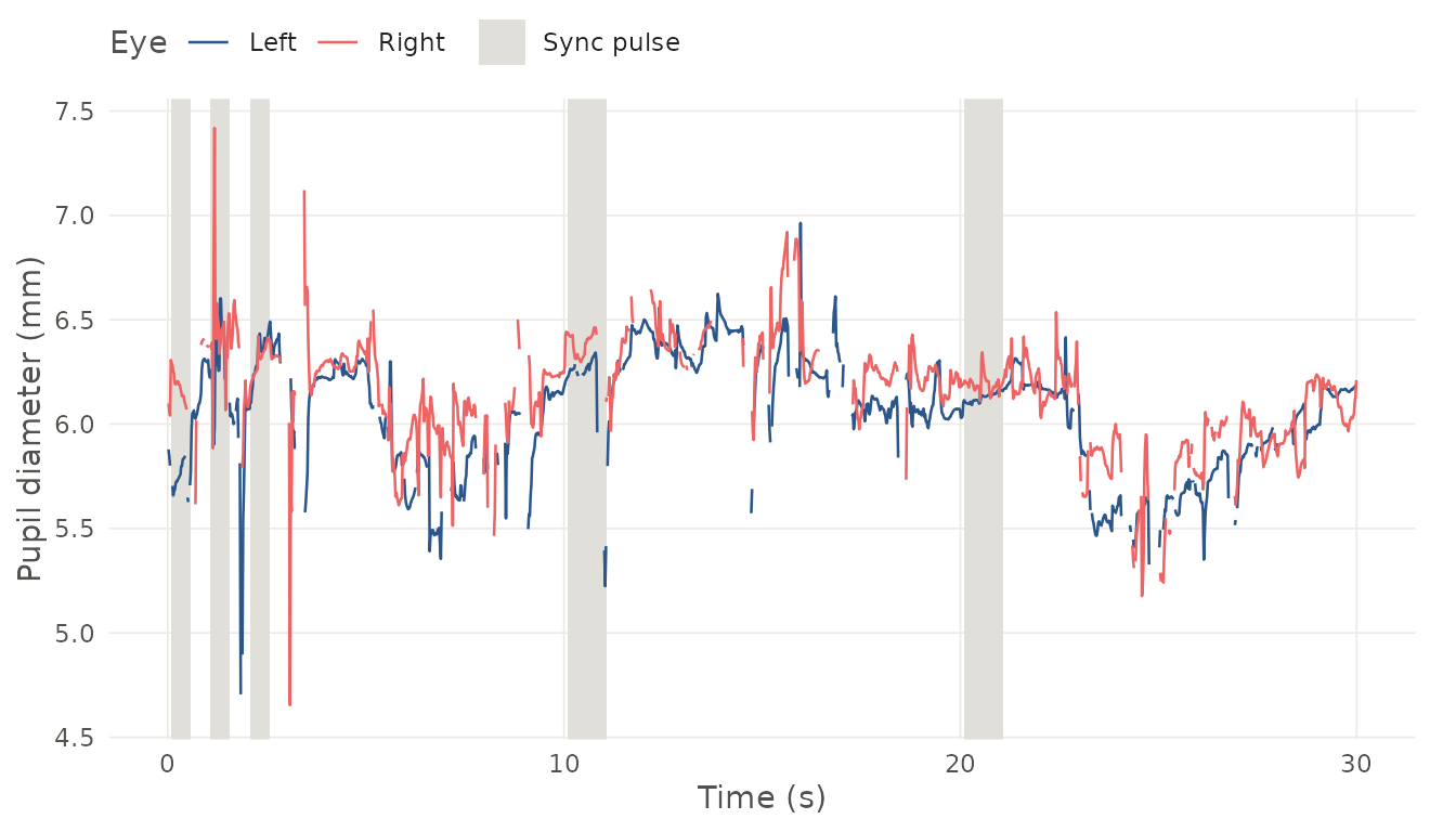
The grey areas mark sync port pulses. The
sync port connects the glasses to other equipment. A stimulus computer
can send a pulse at each stimulus onset, or the glasses can send pulses
that another device records. g3_syncport() lists the pulses
with their onsets and offsets.
g3_syncport(rec$events)
#> # A tibble: 5 × 5
#>   recording pulse   onset offset duration
#>   <chr>     <int>   <dbl>  <dbl>    <dbl>
#> 1 recording     1  0.0785  0.574    0.495
#> 2 recording     2  1.07    1.57     0.499
#> 3 recording     3  2.07    2.57     0.5
#> 4 recording     4 10.1    11.1      0.994
#> 5 recording     5 20.1    21.1      1.000
g3_add_syncport() keeps every sample and adds the sync
port state, the number of the most recent pulse and the time since its
onset. This suits models of the whole recording, where cutting epochs
would drop the samples between pulses.
tagged <- g3_add_syncport(rec$gaze, rec$events)
tagged |>
  filter(syncport == 1) |>
  select(time, pulse, pulse_time)
#> # A tibble: 173 × 3
#>      time pulse pulse_time
#>     <dbl> <int>      <dbl>
#>  1 0.0982     1     0.0197
#>  2 0.118      1     0.0397
#>  3 0.138      1     0.0597
#>  4 0.158      1     0.0798
#>  5 0.178      1     0.0998
#>  6 0.198      1     0.120
#>  7 0.218      1     0.140
#>  8 0.238      1     0.160
#>  9 0.258      1     0.180
#> 10 0.279      1     0.200
#> # ℹ 163 more rows
Long recordings are hard to read at 50 samples per second. The
smooth argument draws a running
median over the raw trace, here one second wide. Short blinks do
not pull it down, and the data themselves are not changed.
plot_g3_pupil(rec, smooth = 1)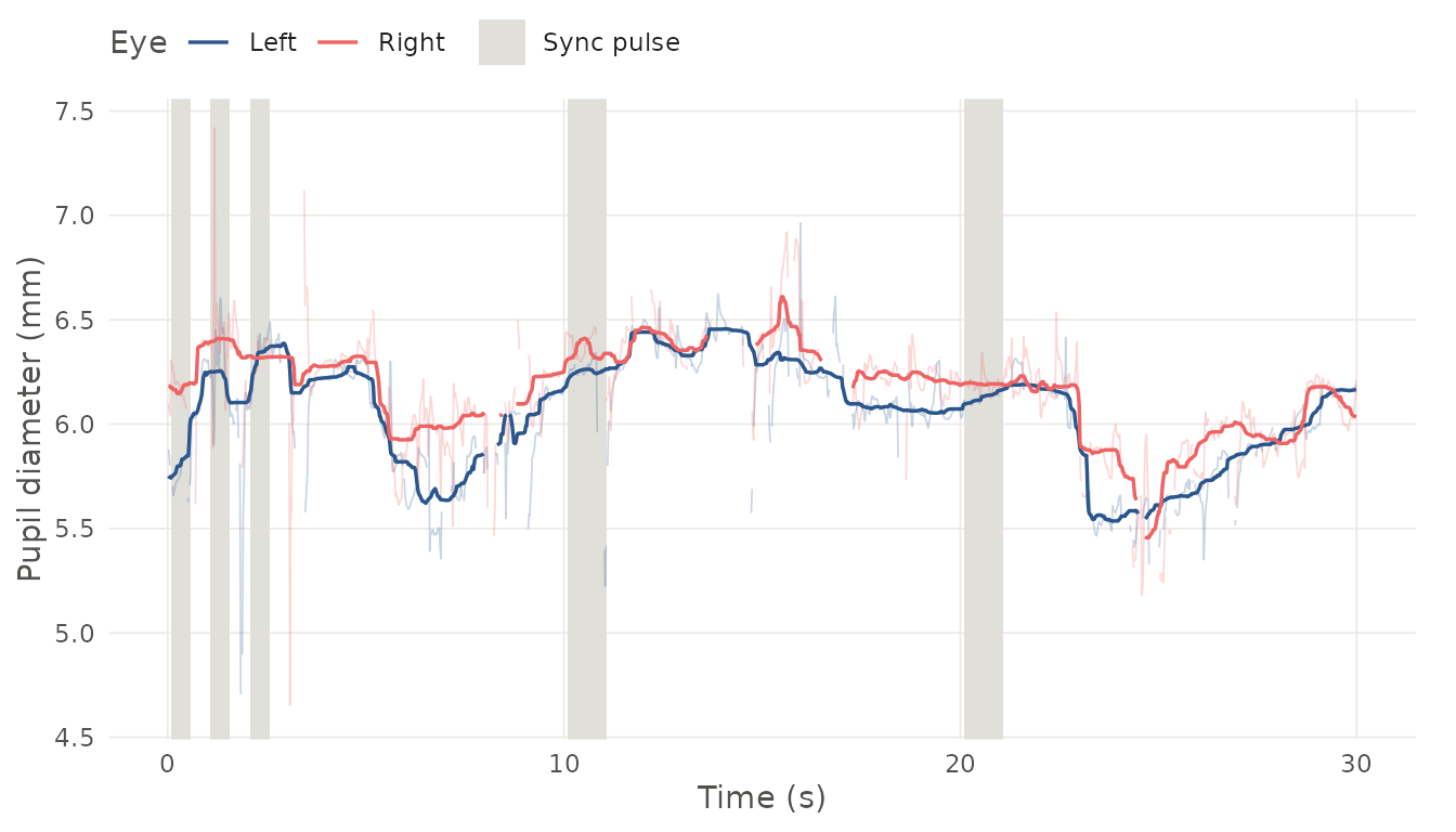
Epochs
g3_epochs() cuts the samples into epochs around each pulse onset and adds the time
relative to the onset. After g3_pupil_long(), there is one
row per sample and eye, which suits ggplot2 and mixed-effects
models.
ep <- g3_epochs(rec$gaze, rec$events, before = 0.5, after = 5)
pupil <- g3_pupil_long(ep)
head(pupil)
#> # A tibble: 6 × 12
#>   recording   time gaze2d_x gaze2d_y gaze3d_x gaze3d_y gaze3d_z valid pulse
#>   <chr>      <dbl>    <dbl>    <dbl>    <dbl>    <dbl>    <dbl> <lgl> <int>
#> 1 recording 0.0180    0.460    0.842     49.0    -208.     549. TRUE      1
#> 2 recording 0.0180    0.460    0.842     49.0    -208.     549. TRUE      1
#> 3 recording 0.0381    0.457    0.846     58.0    -237.     616. TRUE      1
#> 4 recording 0.0381    0.457    0.846     58.0    -237.     616. TRUE      1
#> 5 recording 0.0581    0.455    0.850     70.7    -279.     718. TRUE      1
#> 6 recording 0.0581    0.455    0.850     70.7    -279.     718. TRUE      1
#> # ℹ 3 more variables: epoch_time <dbl>, eye <chr>, pupil <dbl>
Given epochs, plot_g3_pupil() puts the time from the
pulse onset on the x axis. Each eye gets its own panel, with a thin line
per pulse and the mean drawn on top.
plot_g3_pupil(ep)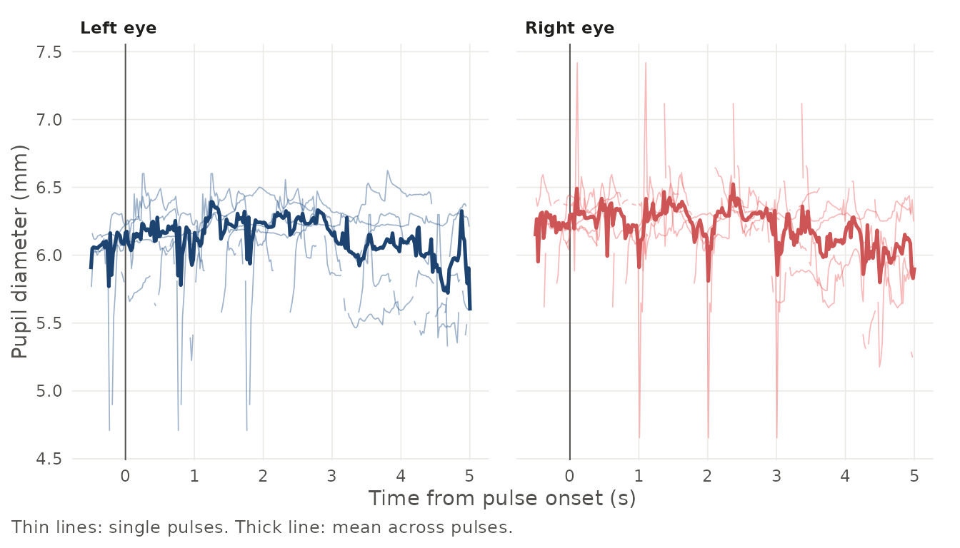
For models of the whole time course, such as generalised additive
mixed models, g3_downsample() averages the samples into
time bins. Bins are counted from the pulse
onset, and a bin where more than half of the samples are missing is left
empty. Character columns, such as a participant or condition label, are
dropped unless you name them in by, and the groups of a
grouped tibble are kept.
binned <- g3_downsample(pupil, bin = 0.1)
head(binned)
#> # A tibble: 6 × 13
#>   recording pulse eye   epoch_time samples   time gaze2d_x gaze2d_y gaze3d_x
#>   <chr>     <int> <chr>      <dbl>   <dbl>  <dbl>    <dbl>    <dbl>    <dbl>
#> 1 recording     1 left        -0.1       4 0.0481    0.454    0.853     65.6
#> 2 recording     1 left         0         5 0.138     0.447    0.869    162.
#> 3 recording     1 left         0.1       4 0.228     0.454    0.866    476.
#> 4 recording     1 left         0.2       5 0.319     0.456    0.884    115.
#> 5 recording     1 left         0.3       5 0.419     0.457    0.907     37.8
#> 6 recording     1 left         0.4       5 0.519     0.414    0.848    174.
#> # ℹ 4 more variables: gaze3d_y <dbl>, gaze3d_z <dbl>, valid <dbl>, pupil <dbl>
glasses3 leaves pupil preprocessing to other packages. PupillometryR, gazer and eyeris handle blink removal, interpolation and baseline correction.
Gaze position
plot_g3_gaze() shows where the wearer looked in the
scene camera image. The top of the plot is the top of the video
frame.
plot_g3_gaze(rec)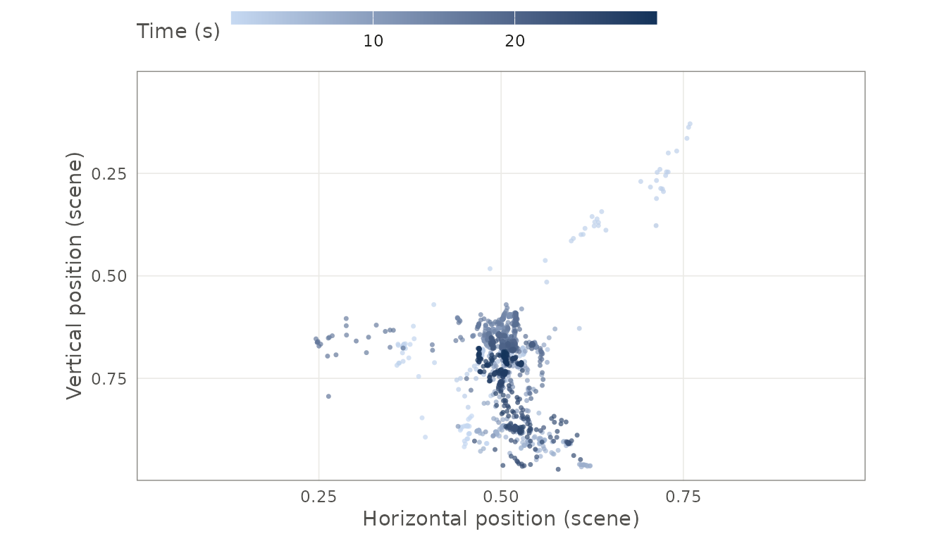
g3_gaze_angles() turns the gaze direction of each eye
into azimuth and elevation in degrees, relative to straight ahead of
the glasses, and adds the vergence angle between
the eyes. Angular velocity for detecting fixations and saccades can be
computed from these columns.
angles <- g3_gaze_angles(rec$gaze)
angles |>
  select(left_azimuth, left_elevation, vergence) |>
  summary()
#>   left_azimuth     left_elevation       vergence
#>  Min.   :-24.647   Min.   :-23.003   Min.   : 0.3509
#>  1st Qu.:  0.685   1st Qu.:-12.245   1st Qu.: 4.2129
#>  Median :  2.172   Median : -7.240   Median : 5.0712
#>  Mean   :  2.015   Mean   : -8.667   Mean   : 5.4612
#>  3rd Qu.:  3.983   3rd Qu.: -5.307   3rd Qu.: 6.1301
#>  Max.   : 25.299   Max.   : 18.841   Max.   :39.3296
#>  NAs    :228       NAs    :228       NAs    :384
Damaged files and gaps
A file that was cut off, for example by an interrupted copy from the
SD card, is still read. The readers skip the damaged lines, return the
intact samples and give a warning that names the skipped lines. A file
whose compressed data are damaged cannot be read and gives an error.
g3_fill_gaps() then inserts empty rows where samples are
missing, so the time series is evenly spaced again before
preprocessing.
filled <- g3_fill_gaps(rec$gaze)
count(filled, inserted)
#> # A tibble: 1 × 2
#>   inserted     n
#>   <lgl>    <int>
#> 1 FALSE     1497
IMU data
The glasses sample the accelerometer and gyroscope together, while the magnetometer runs separately at a lower rate. Each row of the IMU data therefore has missing values for the sensors that were not sampled at that moment.
head(rec$imu)
#> # A tibble: 6 × 11
#>   recording    time accel_x accel_y accel_z gyro_x gyro_y gyro_z mag_x mag_y
#>   <chr>       <dbl>   <dbl>   <dbl>   <dbl>  <dbl>  <dbl>  <dbl> <dbl> <dbl>
#> 1 recording 0.00338  NA       NA      NA      NA    NA      NA   -12.5  31.9
#> 2 recording 0.0119   -0.462   -9.96   -1.69  -17.0  -3.84  -25.3  NA    NA
#> 3 recording 0.0204   -0.527   -9.94   -1.64  -17.6  -4.05  -24.7  NA    NA
#> 4 recording 0.0288   -0.607   -9.87   -1.55  -18.0  -4.37  -24.1  NA    NA
#> 5 recording 0.0373   -0.678   -9.83   -1.52  -18.2  -4.80  -23.3  NA    NA
#> 6 recording 0.0457   -0.722   -9.82   -1.48  -18.4  -5.35  -22.2  NA    NA
#> # ℹ 1 more variable: mag_z <dbl>